Reviewing Cointime Economics
How the new on-chain metrics can be used to quantify the likelihood that bitcoin price levels are (ab)normal

Over the years, on-chain analysis has matured a lot. Institutional-level data providers have come to market, while a lot of very valuable data is also still available for free and utilized by the many analysts in the space. However, it is rare for fundamentally new ideas to emerge. August 24th, 2023, was one of those days on which the field of on-chain analysis was upgraded by a fascinating new concept. David Puell of investment management firm Ark Invest and James Check of data-provider Glassnode published a set of reports (1, 2) called ‘Cointime Economics’, in which they introduce a new approach that sheds new light on a broad set of existing on-chain metrics.
In this article, I will first attempt to reframe the rationale behind Cointime Economics in my own terms, which may hopefully help others to grok the rather abstract concepts in the framework. Then, I will reflect on how the newly introduced metrics may not only be used to estimate ‘fair price’ and ‘floor price’ levels, but also quantify to what extent current or historic market values are (ab)normal.
Why did we need a new approach in the first place?
A lot of the existing on-chain analysis techniques use the bitcoin supply. Since a part of the total bitcoin consists of coins that are (likely) lost (e.g., Satoshi’s coins, coins in lost wallets or provably burned coins), metrics that utilize the bitcoin supply in an attempt to say something useful on current or historic market prices do not optimally reflect those market conditions.
An example of this is the Realized Price (Figure 1; orange) that is derived from the Realized Cap, which was introduced by Nic Carter and Antoine Le Calvez in 2018. The realized price is the dollar value of all bitcoin at the price at which they last moved (= Realized Cap), divided by the total bitcoin supply. The result is a dollar-denominated value that is often described as the market’s average cost basis. Soon after in 2018, Murad Mahmudov and David Puell iterated upon this with the Market Value to Realized Value (MVRV) ratio, by dividing Bitcoin’s Market Cap by the Realized Cap (Figure 2; red). The MVRV ratio therefore reflects the extent in which historic market prices are overextended or undercooled in comparison to the estimated average cost basis of the market, and thus aimed to express to what extent the average market participant is in profit or at a loss.

Since many of the bitcoin that were lost in the early days of the network last moved at very low prices, the calculated realized price is much lower than it would have been if lost coins were excluded. The realized value metric aims to describe the average cost basis of the available bitcoin — since those are the only ones that matter from a market-perspective — but actually provides an underestimation of that number because it uses the total bitcoin supply without accounting for lost coins. Chapter 8 of Glassnode’s report provides several case studies of how many bitcoin may be lost and comes to a best estimate of between 18.5% (3.897M BTC) and 23.2% (4.871M BTC) of the circulating supply. Since the actual number of lost coins is and will remain unknown, there is a need for a different and preferably more dynamic approach. Enter Cointime Economics.
What is the new approach in Cointime Economics?
Cointime Economics iterates on ‘liveliness’ (Figure 2), a metric that was introduced by the late Tamas Blummer in late 2018 and became famous in 2019 for its use in calculating the unrealized profit and loss metrics in a collaboration with Tuur Demeester and Michiel Lescrauwaet. Liveliness itself utilizes another metric called Coin Days Destroyed (CDD), which was one of the first ever on-chain metrics and introduced in 2011. CDD is calculated by taking the number of bitcoin in a transaction and multiplying it by the number of days since those bitcoin were last spent. Hence, CDD is particularly high when a large number of old bitcoin transact, and low when only a limited number of bitcoin that are relatively young move on-chain. Liveliness takes the sum of all CDD, divided by the sum of all coin days that were ever created. Liveliness therefore increases when long term holders liquidate positions and decreases when market participants are increasingly holding onto their bitcoin. It can therefore be seen as a reflection of how willing the bitcoin holder base is to part with their coins.
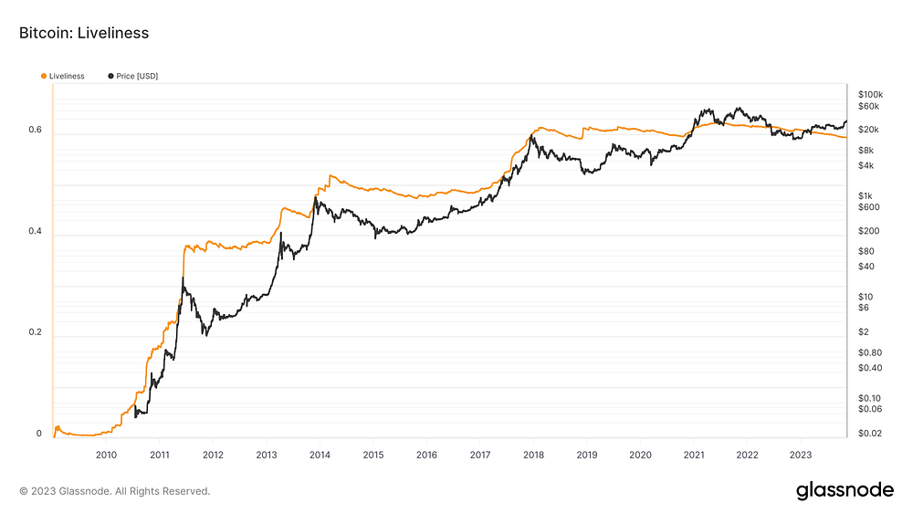
What’s new in Cointime Economics is the concept of ‘Coinblocks’ (Figure 3). Coinblocks are similar to CDD, and are calculated by multiplying the number of coins that are transacted by the number of blocks that have passed since those coins last moved.

Similar to coin days, Coinblocks can also be described as ‘created’, ‘destroyed’ and ‘stored’. The number of Coinblocks created (CBC) simply increases with each newly mined bitcoin that comes into circulation and each block that passes. Coinblocks destroyed (CBD) represent the number of Coinblocks that are wiped out when coins transact on-chain, whereas Coinblocks stored (CBS) represents the number of Coinblocks that were not destroyed (=CBC — CBD).
Tamas Blummer’s liveliness metric can be recalculated by dividing the total number of Coinblocks destroyed by the total number of Coinblocks that were ever created. At a first glance, this finding may seem insignificant, but has the clear advantage that these inputs can now be calculated purely based on inputs that are available on the blockchain itself, which results in a metric that is more accurately reproducible across data providers. Furthermore, it enables the possibility to not only weigh metrics by price but also by time, as we will see in the two new metrics that will be described below.
How was this used to iterate on Realized Price and the MVRV ratio?
As described above, the Realized Price is often interpreted as the market’s average cost basis, but actually represents an underrepresentation of that value because it does not account for lost coins. In Cointime Economics, a new metric was introduced that uses liveliness to weigh the new metric for the extent in which the total market is actually ‘alive’. Because the creators of the new metric chose to do so based on a derivate of the Realized Cap instead of the Realized Cap itself, we will first briefly explain the Thermocap and Investor Cap before diving into the new metric.
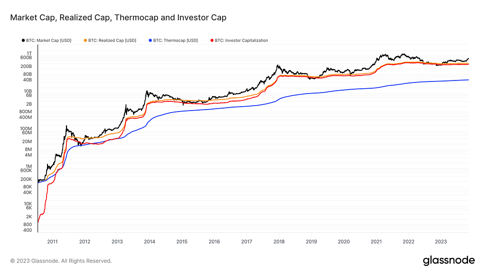
Realized cap is the total price of all existing bitcoin at the price at which they last moved (Figure 4; orange). As a reflection of the total market, this includes both coins that were mined, as well as bought on the market (e.g., at exchanges). The portion of the Market Cap (Figure 4; black) that consists of the value that has been paid to miners to secure the network via the issuance of new coins is called the ‘Thermocap’ (previously introduced by Nic Carter), and can be calculated as the aggregated dollar-value of each bitcoin at the time it was mined (Figure 4; blue). By subtracting the Thermocap from the Market Cap, the ‘Investor Cap’ (previously introduced by Ark Invest) can be found (Figure 4; red). The Investor Cap represents the portion of the total Market Cap that was not introduced via the issuance of new coins by miners, but that actually moved on-chain at a certain market price. As such it is seen as a more appropriate reflection of the average price that was paid for each existing bitcoin by market participants.
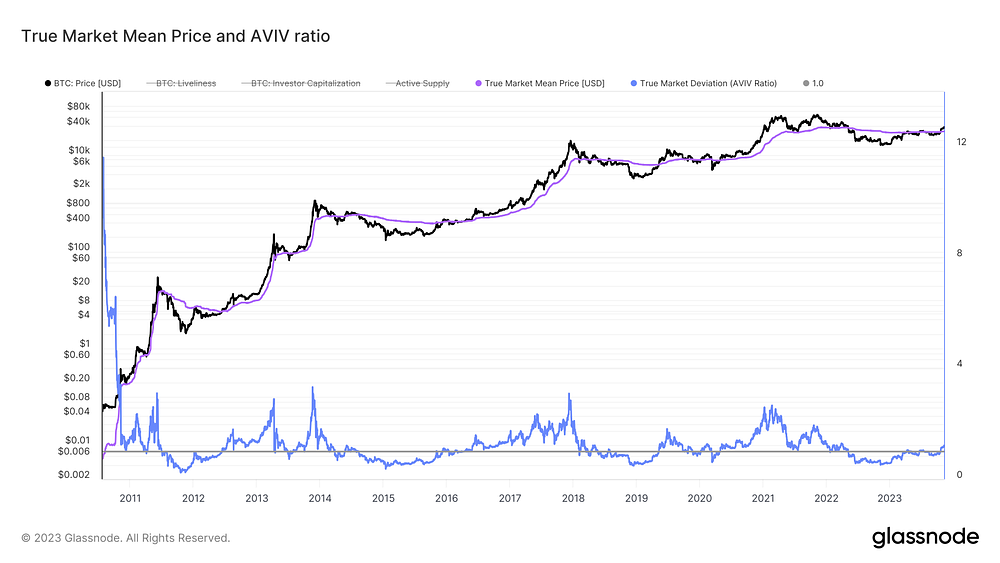
Cointime Economics introduces a new alternative for the Realized Price called the ‘True Market Mean Price’, which is calculated by dividing the Investor Cap that was described above by the Active Supply, which is the total bitcoin supply multiplied by the liveliness (Figure 5; purple).
Similarly to how the MVRV ratio divides the bitcoin Market Cap by the Realized Cap, a new metric that utilizes the Investor Cap and Liveliness-weighted Market Cap was proposed. Puell and Check implicitly proposed the following 2 adaptations to the original MVRV ratio:
- Numerator: Instead of using just the Market Cap, weigh the Market Cap by liveliness (Market Cap * Liveliness) to create a new metric called ‘Active Cap’ that accounts for the extent in which the market can be seen as ‘alive’, and thus dynamically accounts for potentially lost coins.
- Denominator: Instead of dividing this number by the Realized Cap, divide it by the Investor Cap that excludes the portion of the value that was introduced by newly mined coins from the Realized Cap and thus only uses coins that actually moved on-chain at a certain market price.
By doing so, the new metric called Active-Value-to-Investor-Value (AVIV) Ratio (Figure 5; blue) provides a more accurate reflection for the degree in which the average active market participant is in profit or at a loss by dynamically accounting for lost coins. AVIV ratio values above 1 suggest that the market price is above the average active market participant’s cost basis, whereas values below 1 indicate that the average active market participant is at a loss.
What properties of these metrics are interesting?
As expected, the True Market Mean Price is significantly higher than the Realized Price and is positioned much more ‘in the middle’ of historic price action. In fact, according to Chapter 6 of Glassnode’s report, the True Market Mean Price is so ‘in the middle’ that both the mean (1.018) and median (1.038) AVIV ratio values are very close to 1, which is the average active market participant’s estimated break-even point. Historically, the bitcoin price trades above an AVIV ratio value of 1 53.3% of the time, and 46.7% below it. This property makes the AVIV ratio quite unique, and makes the True Market Mean Price an ideal ‘fair value’ estimate as the basis for over- and undervaluation modeling. However, there are two aspects of the AVIV ratio metric that can be improved for use in statistical valuation modeling.
First, the AVIV ratio values during the early days of Bitcoin are incredibly high (Figure 5, blue values on the left). The explanation is simple: after bitcoin received its first price of a few cents in July 2010, the initial exchanges were very illiquid, which was fertile ground for a massive run-up in price — its first hype cycle. One can argue that the AVIV ratio values of that first hype cycle are heavily skewed by market inefficiencies and initial price discovery, and should not be used as part of a historical ‘measuring stick’ to compare more recent values to. A solution could be to only use AVIV ratio values after January 1st, 2012, when the Bitcoin hype cycle went through its first rapid bull-bear cycle, and the average active market participant was just back to its break-even point.
Second, the blue graph in Figure 5 shows that AVIV ratio values fluctuate around 1, but on this linear chart deviate farther away above 1 during bull-runs than they deviate downwards during bear markets. Again, the reason for this is evident: due to how the metric is calculated, the theoretical upside of the scale is infinite, whereas the downside of the scale is 0. For data-visualization purposes this can simply be corrected for by placing the y-axis on a logarithmic scale (as the authors of Cointime Economics have done), but if you want to use this data for statistical calculations, applying the logarithmic transformation to the data itself can be helpful.
In Figure 6, both suggested adaptations were applied. A (natural) logarithmic transformation was performed on the AVIV ratio (blue) values since January 1st, 2012. The AVIV ratio is exactly the same as the regular AVIV ratio when visualized on a logarithmic y-axis (e.g., as depicted on page 18 of Ark Invest’s report), but now fluctuates around a value of 0, where values above 0 signal profitable market conditions and values below 0 suggest that the average active market participant is at a loss.

How can this be used for statistical modeling?
The log-transformed AVIV ratio that we created above represents the degree in which the current average bitcoin market participant is estimated to be in profit (values >0) or at a loss (<0). Even if the AVIV ratio is considered to be the best available model for this, it remains an estimate of the actual average cost basis. The fun thing with statistics is that we can actually express how certain we are that a finding is correct — in this case if historical bitcoin market prices are abnormally discounted or overvalued.
Since the log-transformed AVIV ratio has a distribution that is symmetrical around a mean (of in in this case 0) where values around it are more frequently occurring than values further away from it, it has a ‘normal’ or ‘Gaussian’ distribution. In fact, that is its literal definition according to Investopedia. As a result, the metric can be used for ‘parametric’ statistical analysis, which is a fancy word for the most common form of statistical analysis, often using the variable’s mean and standard deviation. This for instance enables the same z-score based modeling approaches that I’ve written about before (e.g., Bitcoin Price Temperature, MVRV Bands and MVIV + MVLV Bands) — but it will work in a more clean way for the AVIV ratio due to its more appropriate statistical properties.
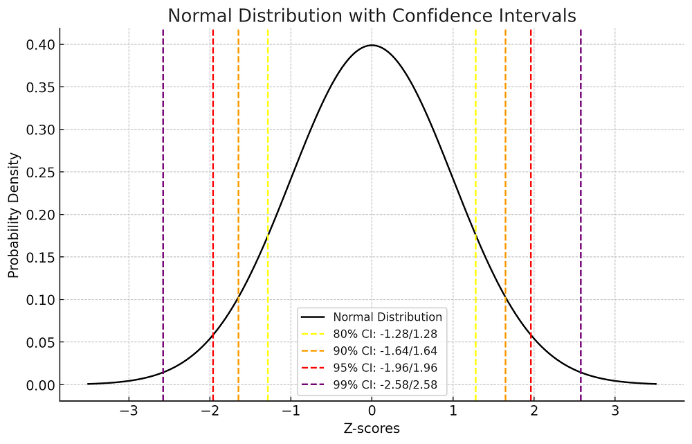
With a normal distribution, we can use z-scores to calculate ‘confidence intervals’. A confidence interval is a range of values that is likely to contain the ‘true answer’ to a question. The ‘null hypothesis’ (/base case) for the log-transformed AVIV ratio is that historical bitcoin market prices are on average at ‘fair value’, as most values tend to be close to 0. The ‘alternate hypothesis’ is that a certain market value is not at fair value and thus abnormally priced. Since bitcoin can be both over- and underpriced in comparison to this ‘fair value’, we need our confidence interval to be two-sided.
Mathematically, we know that in a normal distribution, 95% of the values are within -1.96 and +1.96 standard deviations of the mean. Therefore, when the log-transformed AVIV ratio is 1.96 standard deviations above its mean, we can state that we are 95% certain that bitcoin is abnormally overpriced compared to its fair value. And similarly, when the log-transformed AVIV ratio is 1.96 standard deviations below its mean, the conclusion would be that with 95% certainty, bitcoin is underpriced. This 95% confidence interval is the most common in statistical testing in most academic fields, but the 90%, and to a lesser extent 80% and 99% confidence intervals can also be used (e.g., depending on sample size or expected effect size). Figure 7 shows an example of a normal distribution with two-sided 80%, 90%, 95% and 99% confidence intervals.
Enough theory — what does this look like for AVIV?
Figure 8 [the parameters for the Glassnode Workbench graphs can be found in the Appendix underneath this article] shows a graph of the log-transformed AVIV ratio (black), a zero-line that represents the ‘True Market Mean Price’ (grey), and the 90% and 95% confidence intervals. The confidence intervals are drawn by calculating the all-time rolling mean and standard deviation of the log-transformed AVIV ratio values since January 1st, 2012. By using all-time rolling values, historic values in the graph itself do not change when calculated on different dates, and the confidence intervals gradually adapt, as they widen during increased volatility (in the AVIV ratio values) and tighten if volatility decreases over time. From that perspective they are a bit similar to Bollinger Bands, but more stable over time as they use a much larger and dynamically expanding timeframe.

So far, the 95% confidence intervals for the log-transformed AVIV ratio have signaled both under- and overvalued market prices during each of the 3 market cycles that have occurred since 2012. It is important to realize there are no guarantees that price movements will remain as volatile in the future, and thus that the AVIV ratio values will not necessarily become as abnormal (in both directions) again in the future. However, when it does occur again in the future, we now have a tool that we can use to express how abnormal those prices are in a historical context.
Similarly to how we have utilized z-scores to plot related price levels on the bitcoin price chart for the Bitcoin Price Temperature, MVRV Bands and MVIV + MVLV Bands, we can now also do so based on the log-transformed AVIV ratio values. The result could be called ‘AVIV Confidence Bands’ and is shown in Figure 9.

Just for fun, as an alternative data-visualization, since the Glassnode Workbench software that was used to create these graphs now also allows annotations when a certain condition is met. Figure 10 shows the historical bitcoin price (black) with color-coded annotations when the log-transformed AVIV ratio is below the bottom 90%, 95% or 99% confidence interval (green shades) or the top ones (red shades). This figure shows that historically, it has not always been wise to for instance sell bitcoin as soon as the upper boundaries of the 90% or 95% confidence intervals were reached, as abnormal prices tend to occur over somewhat longer time-periods during both bull- and bear-markets.

Did Cointime Economics introduce other models?
In Cointime Economics, Puell and Check also introduced a new ‘floor model’, that aims to model the ‘price floor’ that the bitcoin price sometime briefly dips below, but always relatively soon bounces back above. The new model, which is described as both the ‘Cointime Price’ and ‘Blummer Price’ by the authors, utilizes the coinblocks that were introduced above. It is calculated by first calculating the all-time cumulative sum of all Cointime Value Destroyed (CVD), and then dividing it by the all-time cumulative sum of all coinblocks destroyed. The rationale behind this has not been as thoroughly documented as the one behind the AVIV ratio, but the model itself does not dissappoint. Figure 10 visualizes the Cointime Price / Blummer Price in green, and shows that it is consistently lower than the Realized Price (orange).

Can confidence intervals also be used for this?
In the introduction to confidence intervals above, we reflected on the situation where the null hypothesis was that the bitcoin market price is around ‘fair value’, and can deviate from it in both directions. In the case of the Cointime Price / Blummer Price, the basic premise is that the floor model represents the bottom of the price range, and thus that market values can only abnormally deviate from it to the upside. For this situation, it is possible to use one-sided confidence intervals, for which slightly different z-scores are used. In the same style as the normal distribution with two-sided confidence intervals was displayed in Figure 7, Figure 12 shows an example distribution that utilizes one-sided confidence intervals.

To properly align with the approach that we used for the log-transformed AVIV Ratio above, we first need to calculate a similar indicator to the AVIV ratio. Since we want to estimate to what extent the current market value is overvalued against the floor price of the Cointime Price / Blummer Price, we can calculate the Market-Value-to-Cointime-Value (MVPV) or Market-Value-to-Cointime-Value (MVBV) ratio by simply dividing the bitcoin market price by the Cointime Price / Blummer Price. Then we plot the one-sided confidence intervals by first calculating the all-time rolling mean and standard deviation of this new metric, and plotting the lines on the chart (rolling mean + [z-score of the one-sided confidence interval] * rolling standard deviation), as is done in Figure 13.
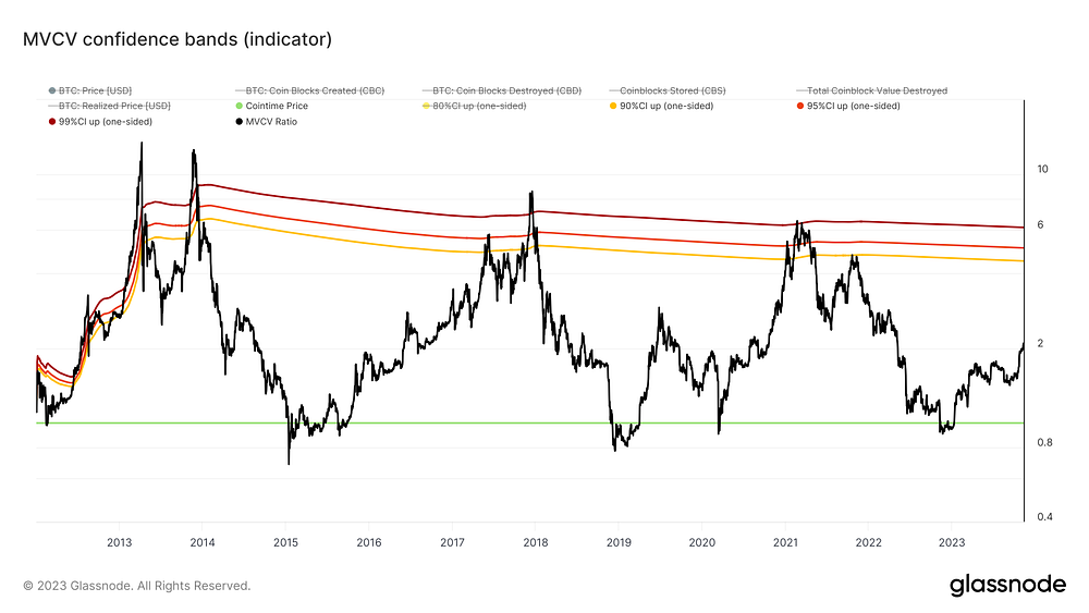
Similar to before, these confidence intervals can also be plotted on the price chart (Cointime Price + z-score * all-time rolling standard deviation of MVPV ratio) in Figure 14.

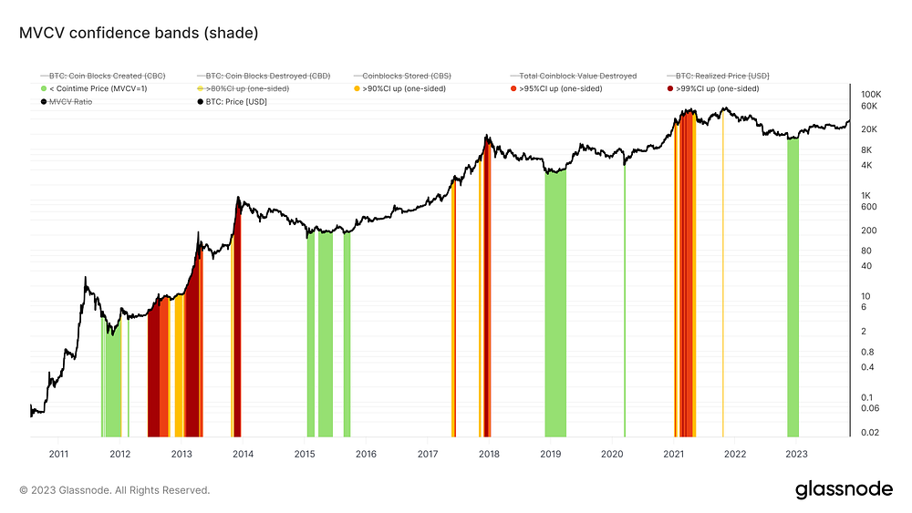
To close off, the MVCV/MVBV ratio and confidence bands can also be plotted using the color-coded annotations that we utilized above for the AVIV ratio, as is done in Figure 15.
Are there any caveats with this approach?
There are several differences between the approaches used for the log-transformed AVIV ratio and MVCV/MVBV confidence bands:
- The fundamental reasoning behind the AVIV ratio has been more clearly described than for the Cointime Price / Blummer Price.
- The assumption that market value can be expected to stick close to the AVIV ratio based ‘fair value’ (basically; mean reversion) appears to be more fundamentally sound than the assumption that the market value should not dip far and/or long below the Cointime Price / Blummer Price floor model.
- An approach that utilizes two-sided intervals (e.g., admitting that we don’t know in what price can or cannot deviate from its fair value) is more conservative than one that assumes value can only deviate up.
As such, I personally see the AVIV ratio and related models that were discussed above as more fundamentally sound and trustworthy than the Cointime Price / Blummer Price related models.
In both cases, it is important to realize that historic price movements and -volatility do not necessarily reoccur in the future. Although the bitcoin price has historically moved eerily consistent on a 4-year cycle that appears to be related to the halving schedule (and/or the global liquidity cycle that has been flowing with a similar beat since Bitcoin was born), it is also reasonable to expect that as a result of the maturing market, volatility should be expected to gradually become less extreme.
The confidence intervals and bands that were introduced in this article may appear to represent hard cut-off points for when the bitcoin market cycle should be expected to bottom or top, but there are no such clear limits in reality — especially during extreme bear- or bull-market conditions where fear and FOMO tend to skew rational thinking. Similar to how some academic fields are moving from a traditionally ‘frequentist’ (e.g., drawing binary conclusions depending on if a value is above or below a pre-set threshold, e.g. p<.05) to a ‘Bayesian’ approach (e.g., using available evidence to estimate the probability of a certain result being true), it is healthy to interpret these metrics with a more probabilistic mindset when aiming to analyze the market, ideally in combination with other metrics.
Appendix: Glassnode Workbench parameters
Required: Glassnode Tier 2 subscription
Figure 8 — AVIV confidence bands (indicator)
Metrics: [m1] BTC: Price; [m2] BTC: Liveliness; [m3] BTC: Circulating Supply; [m4] BTC: Investor Capitalization
Formulae: [f1] f10-f10; [f2] cummean(f10) + 2.57 * cumstd(f10); [f3] cummean(f10) + 1.96 * cumstd(f10); [f4] cummean(f10) + 1.64 * cumstd(f10); [f5] cummean(f10) + 1.28 * cumstd(f10); [f6] cummean(f10) -1.28 * cumstd(f10); [f7] cummean(f10) -1.64 * cumstd(f10); [f8] cummean(f10) -1.96 * cumstd(f10); [f9] cummean(f10) -2.57 * cumstd(f10); [f10] log(subset(m2*m3*m1/m4, “2012”, “2099”))
Figure 9 — AVIV confidence bands (price)
Metrics: [m1] BTC: Liveliness; [m2] BTC: Circulating Supply; [m3] BTC: Investor Capitalization; [m4] BTC: Price
Formulae: [f1] m3/(m1*m2); [f2] log(subset(m1*m2*m4/m3, “2012”, “2099”)); [f3] (2.7182818284590452353602874713527^(cummean(f2) + 2.57 * cumstd(f2)))*f1; [f4] (2.72^(cummean(f2) + 1.96 * cumstd(f2)))*f1
[f5] (2.7182818284590452353602874713527^(cummean(f2) + 1.96 * cumstd(f2)))*f1; [f6] (2.7182818284590452353602874713527^(cummean(f2) + 1.64 * cumstd(f2)))*f1; [f7] (2.7182818284590452353602874713527^(cummean(f2) + 1.28 * cumstd(f2)))*f1; [f8] (2.7182818284590452353602874713527^(cummean(f2) -1.28 * cumstd(f2)))*f1; [f9] (2.7182818284590452353602874713527^(cummean(f2) -1.64 * cumstd(f2)))*f1; [f10] (2.7182818284590452353602874713527^(cummean(f2) -1.96 * cumstd(f2)))*f1; [f10] (2.7182818284590452353602874713527^(cummean(f2) -2.57 * cumstd(f2)))*f1
Figure 10 — AVIV confidence bands (shade)
Metrics: [m1] BTC: Liveliness; [m2] BTC: Circulating Supply; [m3] BTC: Investor Capitalization; [m4] BTC: Price
Formulae: [f1] m3/(m1*m2); [f2] log(subset(m1*m2*m4/m3, “2012”, “2099”)); [f3] m4*if(m4,”>”,((2.7182818284590452353602874713527^(cummean(f2) + 1.28 * cumstd(f2)))*f1),1,0); [f4] m4*if(m4,”>”,((2.7182818284590452353602874713527^(cummean(f2) + 1.64 * cumstd(f2)))*f1),1,0); [f5] m4*if(m4,”>”,((2.7182818284590452353602874713527^(cummean(f2) + 1.96 * cumstd(f2)))*f1),1,0); [f6] m4*if(m4,”>”,((2.7182818284590452353602874713527^(cummean(f2) + 2.57 * cumstd(f2)))*f1),1,0); [f7] m4*if(m4,”<”,((2.7182818284590452353602874713527^(cummean(f2) -1.28 * cumstd(f2)))*f1),1,0); [f8] m4*if(m4,”<”,((2.7182818284590452353602874713527^(cummean(f2) -1.64 * cumstd(f2)))*f1),1,0); [f9] m4*if(m4,”<”,((2.7182818284590452353602874713527^(cummean(f2) -1.96 * cumstd(f2)))*f1),1,0); [f10] m4*if(m4,”<”,((2.7182818284590452353602874713527^(cummean(f2) -2.57 * cumstd(f2)))*f1),1,0)
Figure 13 — MVCV confidence bands (indicator)
Metrics: [m1] BTC: Price; [m2] BTC: Coin Blocks Created (CBC); [m3] BTC: Coin Blocks Destroyed (CBD)
Formulae: [f1] m2-m3; [f2] cumsum(m1*m3); [f3] f8/f8; [f4] cummean(f8) + 0.84 * cumstd(f8); [f5] cummean(f8) + 1.28 * cumstd(f8); [f6] cummean(f8) + 1.65 * cumstd(f8); [f7] cummean(f8) + 2.33 * cumstd(f8); [f8] m1/subset(f2/cumsum(f1), “2012")
Figure 14 — MVCV confidence bands (price)
Metrics: [m1] BTC: Coin Blocks Created (CBC); [m2] Coin Blocks Destroyed (CBD); [m3] BTC: Price
Formulae: [f1] m1-m2; [f2] cumsum(m3*m2); [f3] f2/cumsum(f1); [f4] (cummean(f8) + 0.84 * cumstd(f8))*f3; [f5] (cummean(f8) + 1.28 * cumstd(f8))*f3; [f6] (cummean(f8) + 1.65 * cumstd(f8))*f3; [f7] (cummean(f8) + 2.33 * cumstd(f8))*f3; [f8] m3/subset(f2/cumsum(f1), “2012”)
Figure 15 — MVCV confidence bands (shade)
Metrics: Metrics: [m1] BTC: Coin Blocks Created (CBC); [m2] Coin Blocks Destroyed (CBD); [m3] BTC: Price
Formulae: [f1] m1-m2; [f2] cumsum(m3*m2); [f3] m3*if(m3,”>”,((cummean(f6) + 1.28 * cumstd(f6)))*(f2/cumsum(f1)),1,0); [f4] m3*if(m3,”>”,((cummean(f6) + 1.65 * cumstd(f6)))*(f2/cumsum(f1)),1,0); [f5] m3*if(m3,”>”,((cummean(f6) + 2.33 * cumstd(f6)))*(f2/cumsum(f1)),1,0); [f6] m3/subset(f2/cumsum(f1), “2012")
